Motivation
- Evaluate dynamic predictions of imminent delivery in pregnancies complicated by early-onset fetal growth restriction
- Main goal: optimizing antenatal corticosteroid (CCS) administration

- Methods are applied to data from the OPTICORE multicenter cohort study
Asymmetric misclassification

TP
FP
TN
FN
Definitions and notation
- \(i=1,\dotsc,n\) individuals
- \(\require{color}\textcolor{#EB589A}{T_1^*,\dots, T_n^*}\) true time until event
- \(\require{color}\textcolor{#EB589A}{C_1,\dots, C_n}\) right-censoring times
- \(\require{color}\textcolor{#EB589A}{T_i=\min(T_i^*, C_i)}\) observed times
- \(\require{color}\textcolor{#EB589A}{\delta_i=\mathbf{1}\{T_i^*\leq C_i\}}\) censoring indicator
- \(\require{color}\textcolor{#EB589A}{L_1,\dots, L_n}\) left-truncation times
- \(\require{color}\textcolor{#EB589A}{\boldsymbol{\mathcal{H}}_i(t)}\) available history at time \(t\)
- Dynamic predictions
\[ \normalsize\require{color} \pi_{i}(s \mid t)=\operatorname{Pr}\left(T_{i}^* \leq t+s \mid T_{i}^*>t, \colorbox{#EB589A}{$\color{#FBE1EE}\boldsymbol{\mathcal{H}}_i(t)$}\right) \]

Scoring rules


- A scoring rule is proper if
\[ E\left[\mathcal{S}\big(\pi_i^{\text{true}}(s\mid t), D_i(t,s)\big) \right] \leq E\left[\mathcal{S}\big(\widehat{\pi}_i(s\mid t), D_i(t,s)\big) \right] \]
- It is strictly proper if it holds with equality if and only if \(\pi_i^{\text{true}}(s\mid t)\equiv \widehat{\pi}_i(s\mid t)\)
- It is centered if \(\mathcal{S}(1,1)=\mathcal{S}(0,0)=0\)

Clinical utility
- Focus on the quality of decisions driven by dynamic predictions
- Based on a clinically relevant decision threshold \(c\in(0,1)\)

- A widely used clinical utility metric is the net benefit (NB)
- A similar metric is the expected cost (EC)
- We define the dynamic EC \[ \normalsize\require{color}\begin{split} \begin{split} \text{EC}_c\big(\pi_i(s\mid t),\, & D_i(t,s)\big) = c\mathbf{1}\{\pi_i(s\mid t)\geq c\} (1-D_i(t,s))\\ &+(1-c)\mathbf{1}\{\pi_i(s\mid t)< c\}D_i(t,s) \end{split} \end{split} \]
- A widely used clinical utility metric is the net benefit (NB)
- A similar metric is the expected cost (EC)
- We define the dynamic EC \[ \normalsize\require{color}\begin{split} \begin{split} \text{EC}_c\big(\pi_i(s\mid t),\, & D_i(t,s)\big) = c\textcolor{#EB589A}{\mathbf{1}\{\pi_i(s\mid t)\geq c\} (1-D_i(t,s))}\\ &+(1-c)\mathbf{1}\{\pi_i(s\mid t)< c\}D_i(t,s) \end{split} \end{split} \]
- A widely used clinical utility metric is the net benefit (NB)
- A similar metric is the expected cost (EC)
- We define the dynamic EC \[ \normalsize\require{color}\begin{split} \begin{split} \text{EC}_c\big(\pi_i(s\mid t),\, & D_i(t,s)\big) = \textcolor{#EB589A}{c\mathbf{1}\{\pi_i(s\mid t)\geq c\} (1-D_i(t,s))}\\ &+(1-c)\mathbf{1}\{\pi_i(s\mid t)< c\}D_i(t,s) \end{split} \end{split} \]
- A widely used clinical utility metric is the net benefit (NB)
- A similar metric is the expected cost (EC)
- We define the dynamic EC \[ \normalsize\require{color}\begin{split} \text{EC}_c\big(\pi_i(s\mid t),\, & D_i(t,s)\big) = c\mathbf{1}\{\pi_i(s\mid t)\geq c\} (1-D_i(t,s))\\ &+(1-c)\textcolor{#EB589A}{\mathbf{1}\{\pi_i(s\mid t)< c\}D_i(t,s)} \end{split} \]
- A widely used clinical utility metric is the net benefit (NB)
- A similar metric is the expected cost (EC)
- We define the dynamic EC \[ \normalsize\require{color}\begin{split} \text{EC}_c\big(\pi_i(s\mid t),\, & D_i(t,s)\big) = c\mathbf{1}\{\pi_i(s\mid t)\geq c\} (1-D_i(t,s))\\ &+\textcolor{#EB589A}{(1-c)\mathbf{1}\{\pi_i(s\mid t)< c\}D_i(t,s)} \end{split} \]

- NB and EC rely on a single decision threshold \(c\in (0,1)\)
Integrated weighted expected cost
- To avoid reliance on a single \(c\) and achieve strict properness we define the IWEC
\[\normalsize\require{color}\begin{split} & \text{IWEC}_w \big(\pi_i(s\mid t), D_i(t,s)\big) = \\ & \int_0^1\text{EC}_c\big(\pi_i(s\mid t),D_i(t,s)\big)w(c)dc \end{split} \]
- \(w(\cdot)\) is a positive weight function reflecting the clinical relevance of different \(c\)’s
- To avoid reliance on a single \(c\) and achieve strict properness we define the IWEC
\[\normalsize\require{color}\begin{split} & \text{IWEC}_w \big(\pi_i(s\mid t), D_i(t,s)\big) = \\ & \textcolor{#EB589A}{\int_0^1}\text{EC}_c\big(\pi_i(s\mid t),D_i(t,s)\big)\textcolor{#EB589A}{w(c)dc} \end{split} \]
- We consider the beta family of weight functions \(w(c;\alpha,\beta)\)

- We rely on a weight function, considering all thresholds \(c\in (0,1)\) and its relative clinical importance
- A scoring rule is centered strictly proper \(\Longleftrightarrow\) it can be represented by \(\text{IWEC}_w \big(\pi_i(s\mid t), D_i(t,s)\big)\) for some \(w(\cdot)\)
- For \(w(c)=1\), we obtain the dynamic Brier score
- For \(w(c)=c^{-1}(1-c)^{-1}\), we obtain the dynamic logarithmic score
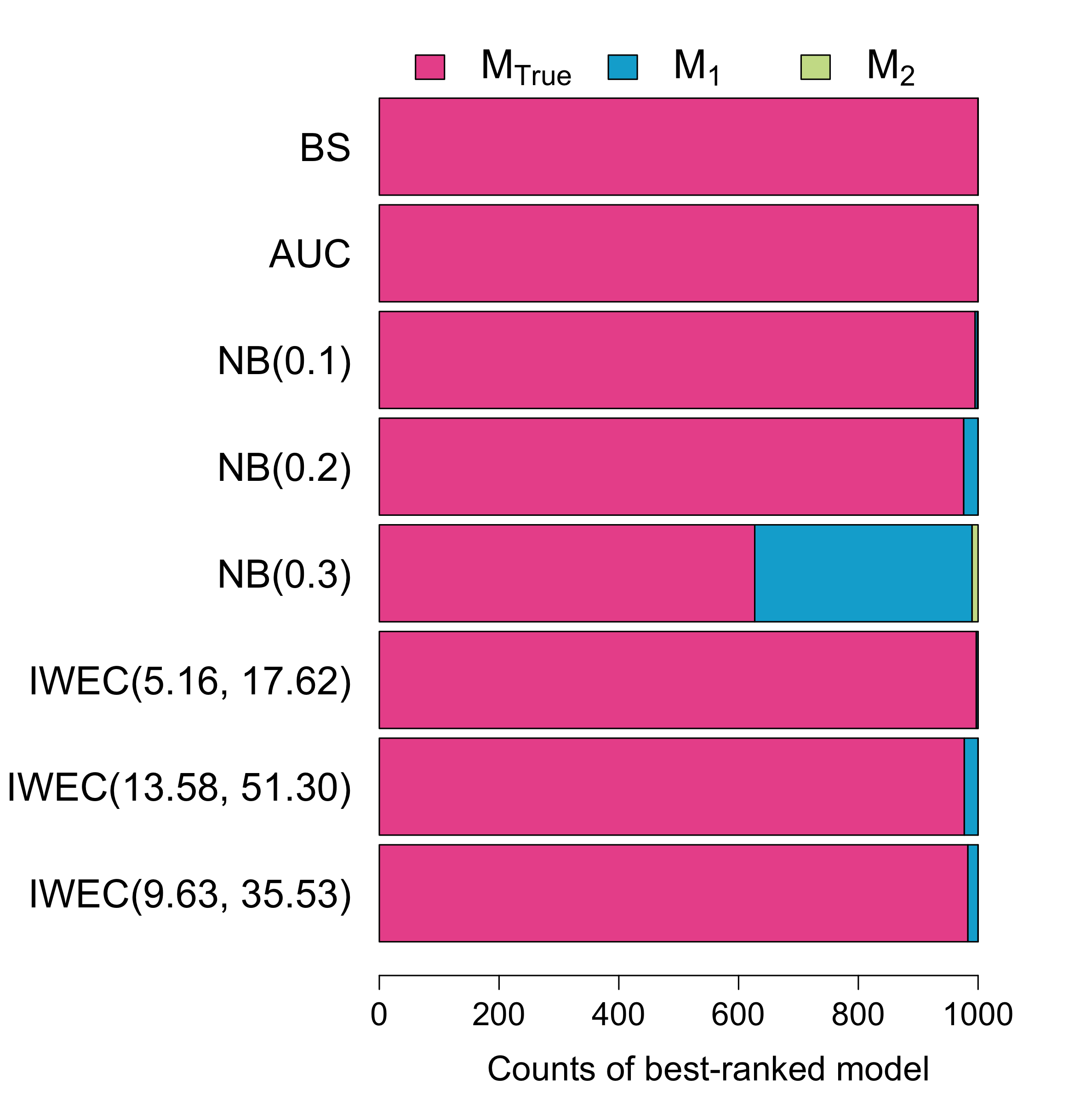
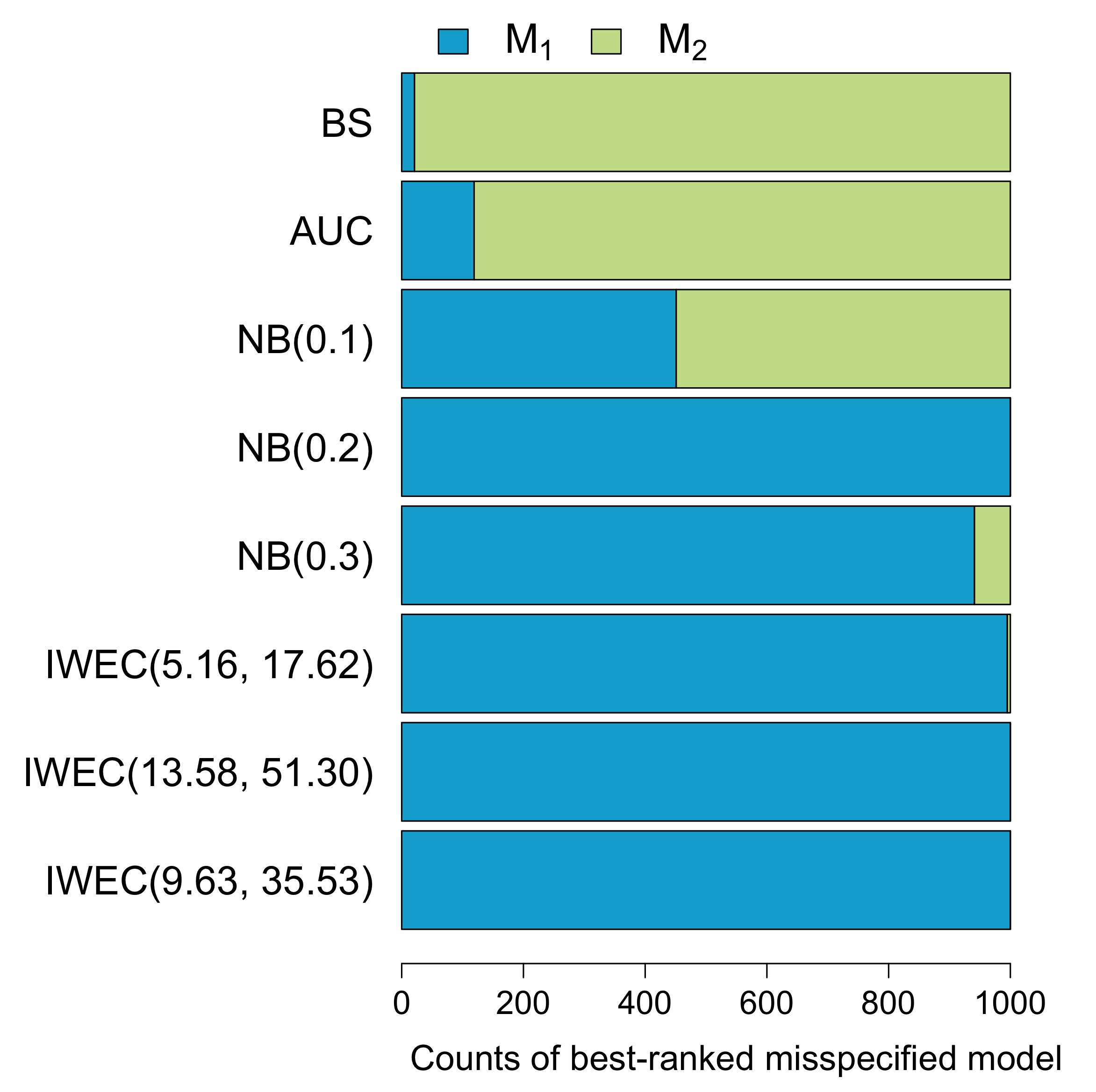
Simulation study
- We evaluate dynamic predictions within \((1,3]\) obtained via three Cox proportional-hazards models:
- The true model \(\longrightarrow\) \(M_\text{True}\)
- Two misspecified models \(\longrightarrow\) \(M_1, M_2\)
- To reflect the asymmetry between FP and FN in our clinical context, we set \(c\in(0.1, 0.3)\)


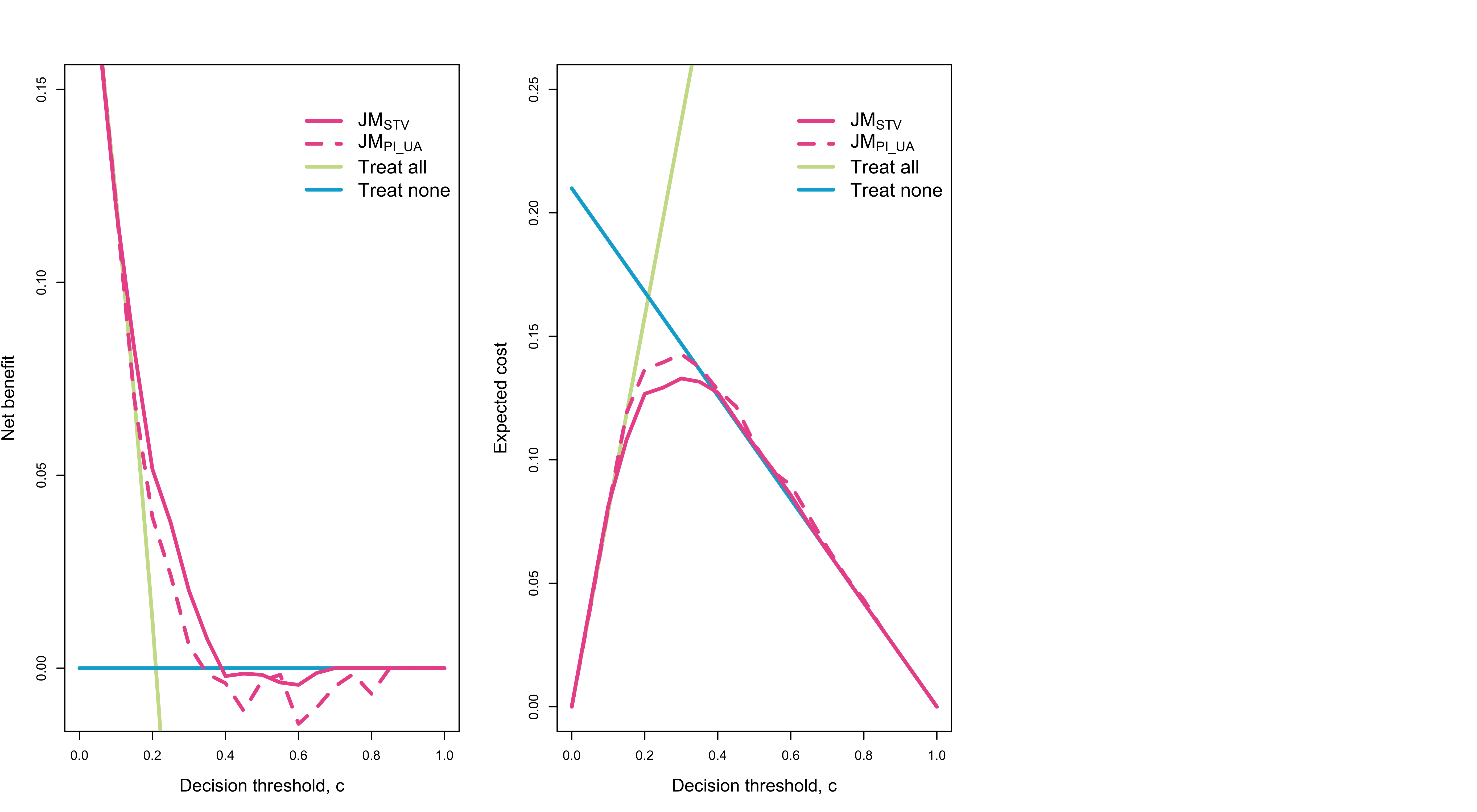
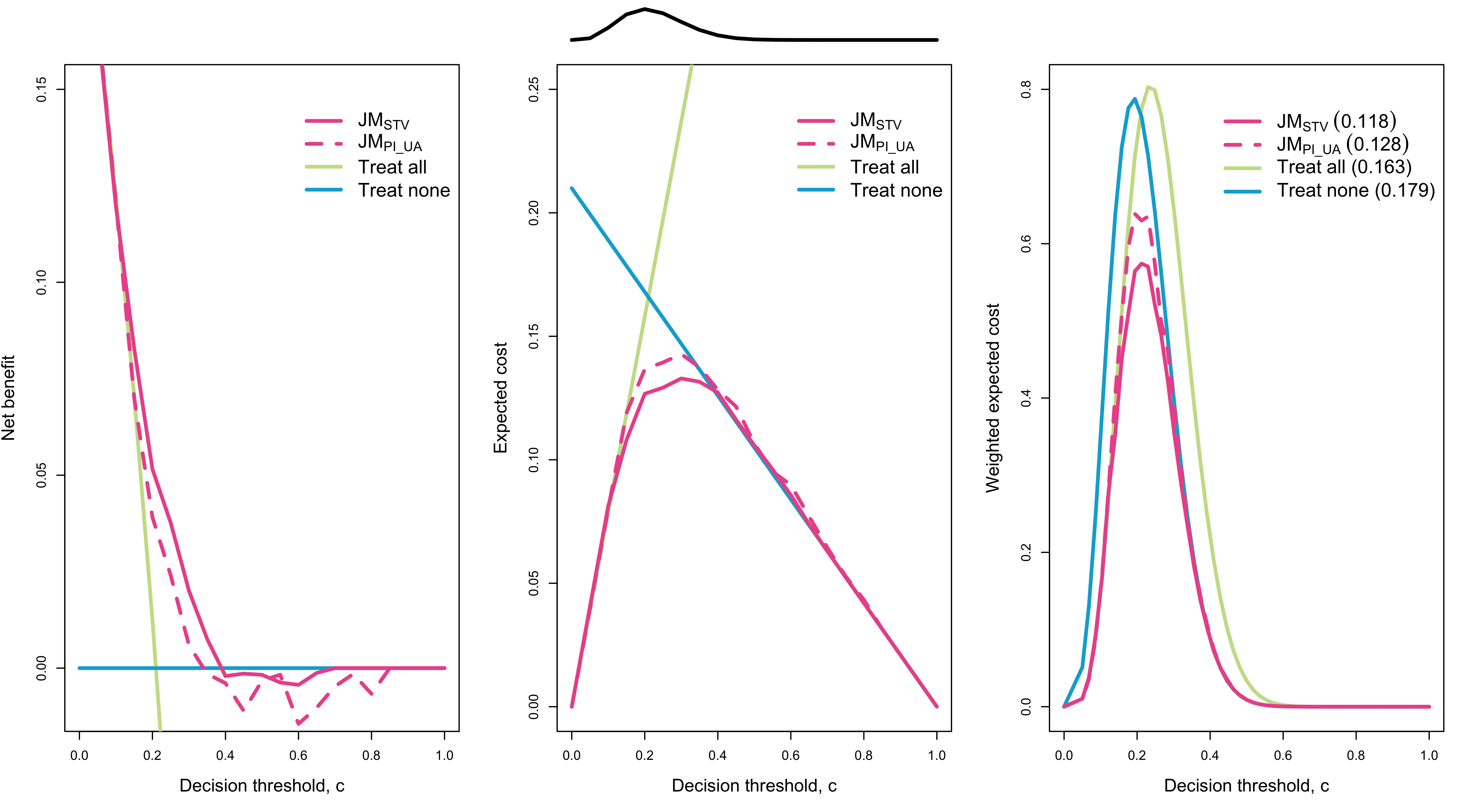
Application: OPTICORE
- Baseline covariates: age, previous pregnancy outcomes, smoking status, pre-existent use of antihypertensive agents, diabetes mellitus, etc.
- We consider fetal longitudinal biomarkers:
- Pulsatility index of the umbilical artery (\(\texttt{PI_UA}\))
- Short-term heart-rate variability (\(\texttt{STV}\))
- Linear mixed-effects submodels:
\[ \require{color}\scriptsize\begin{cases} \texttt{PI_UA}_i(t) & = \colorbox{#EB589A}{$\color{#FBE1EE}m_{1i}(t)$} + \varepsilon_{1i}(t) \\ &= (\beta_0^1 + b_{0i}^1) + (\beta_{1}^1 + b_{1i}^1)B_1^1(t,\lambda) + (\beta_{2}^1 + b_{2i}^1)B_2^1(t,\lambda) + \varepsilon_{1i}(t)\\ \\ \log(\texttt{STV}_i(t)) & = \colorbox{#EB589A}{$\color{#FBE1EE}m_{2i}(t)$} + \varepsilon_{2i}(t)\\ & = (\beta_0^2 + b_{0i}^2) + (\beta_{1}^2 + b_{1i}^2)B_1^2(t,\lambda) + (\beta_{2}^2 + b_{2i}^2)B_2^2(t,\lambda) + \varepsilon_{2i}(t) \end{cases},\]
- Shared-parameter joint models using the same baseline data \(\boldsymbol{X}_i\) and the two longitudinal submodels:
\[\scriptsize\begin{split} \textcolor{#EB589A}{\text{JM}_{\text{PI_UA}}}: & h_{i}\left(t \mid \boldsymbol{\mathcal{H}}_{i}(t), \boldsymbol{X}_{i}\right) =h_{0}(t) \exp \big( \gamma\boldsymbol{X}_{i} + \alpha_1\colorbox{#EB589A}{$\color{#FBE1EE}\frac{m_{1i}(t) - m_{1i}(t-7)}{7}$} \big) \\ \textcolor{#EB589A}{\text{JM}_{\text{STV}}}: & h_{i}\left(t \mid \boldsymbol{\mathcal{H}}_{i}(t), \boldsymbol{X}_{i}\right) =h_{0}(t) \exp \big( \gamma\boldsymbol{X}_{i} + \alpha_2\colorbox{#EB589A}{$\color{#FBE1EE}\frac{1}{7}\int_{t-7}^tm_{2i}(s)ds$} \big) \end{split}\]
- We evaluate dynamic predictions within \((200, 207]\) days of gestation. We still consider \(c\in(0.1,0.3)\), we use \(w(c;5.16, 17.62)\)
- We extend the classical decision curve analysis by defining weighted decision curves
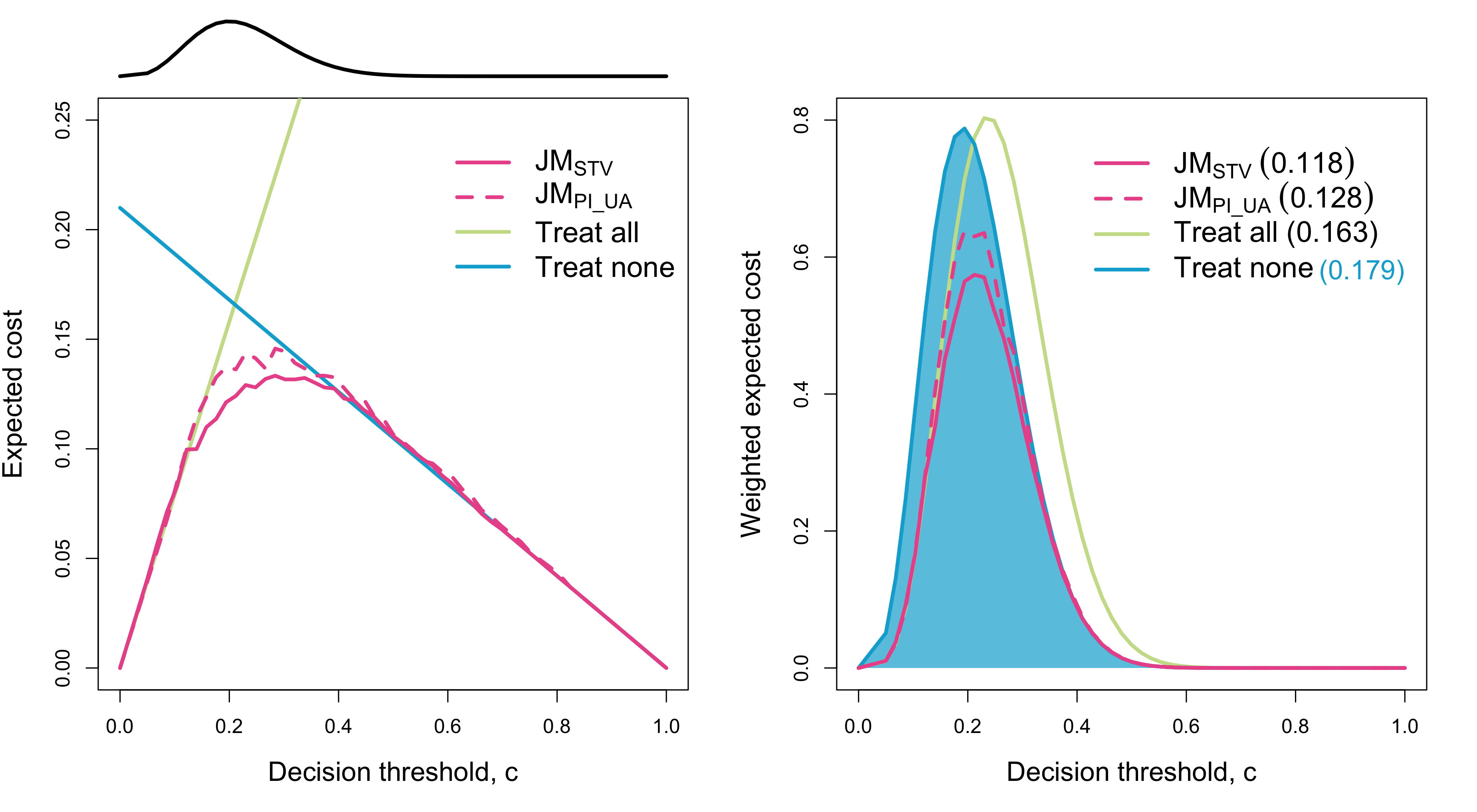


Contribution
- Extension of clinical utility measures (NB and EC) to dynamic prediction
- Dynamic IWEC definition and weighted decision curves
- IPW estimator tailored to LTRC data
- All methods will be available in the JMbayes2 R package
Challenges of the data
- CCS cannot be administered until the fetus reaches \(500\) grams and a gestational age of \(168\) days (\(24\) weeks)

IPW estimator
- Under LTRC data \(D_i(t,s)=\mathbf{1}\{t<T_i^*\leq t+s\}\) is unobserved for \(i\) censored within \((t, t+s]\) or \(L_i>t\)

- Under LTRC data \(D_i(t,s)=\mathbf{1}\{t<T_i^*\leq t+s\}\) is unobserved for \(i\) censored within \((t, t+s]\) or \(L_i>t\)

- We address this problem defining the IPW estimator
\[\require{color} \widehat{\text{eIWEC}_w}(t,s)=\frac{1}{n_t} \sum_{i=1}^n \widehat{W}_i(t,s)\text{IWEC}_w\big(\pi_i(s\mid t),\tilde{D}_i(t,s)\big)\]
- \(n_t\) number of individuals at risk at \(t\)
- \(\tilde{D}_i(t,s)\) the observed binary indicator
- \(\widehat{W}_i(t,s)\) adjust for LTRC data via left-truncated Kaplan–Meier of the censoring distribution
- We address this problem defining the IPW estimator
\[ \require{color}\widehat{\text{eIWEC}_w}(t,s)=\frac{1}{\textcolor{#EB589A}{n_t}} \sum_{i=1}^n \widehat{W}_i(t,s)\text{IWEC}_w\big(\pi_i(s\mid t),\tilde{D}_i(t,s)\big)\]
- \(\textcolor{#EB589A}{n_t}\) number of individuals at risk at \(t\)
- \(\tilde{D}_i(t,s)\) the observed binary indicator
- \(\widehat{W}_i(t,s)\) adjust for LTRC data via left-truncated Kaplan–Meier of the censoring distribution
- We address this problem defining the IPW estimator
\[\require{color} \widehat{\text{eIWEC}_w}(t,s)=\frac{1}{n_t} \sum_{i=1}^n \widehat{W}_i(t,s)\text{IWEC}_w\big(\pi_i(s\mid t),\textcolor{#EB589A}{\tilde{D}_i(t,s)}\big)\]
- \(n_t\) number of individuals at risk at \(t\)
- \(\textcolor{#EB589A}{\tilde{D}_i(t,s)}\) the observed binary indicator
- \(\widehat{W}_i(t,s)\) adjust for LTRC data via left-truncated Kaplan–Meier of the censoring distribution
- We address this problem defining the IPW estimator
\[\require{color} \widehat{\text{eIWEC}_w}(t,s)=\frac{1}{n_t} \sum_{i=1}^n \textcolor{#EB589A}{\widehat{W}_i(t,s)}\text{IWEC}_w\big(\pi_i(s\mid t),\tilde{D}_i(t,s)\big)\]
- \(n_t\) number of individuals at risk at \(t\)
- \(\tilde{D}_i(t,s)\) the observed binary indicator
- \(\textcolor{#EB589A}{\widehat{W}_i(t,s)}\) adjust for LTRC data via left-truncated Kaplan–Meier of the censoring distribution
- We demostrated that
- \(\widehat{\text{eIWEC}_w}(t,s)\) is a consistent estimator of \(\text{eIWEC}_w(t,s)\)
- \(\sqrt{n}\big(\widehat{\text{eIWEC}_w}(t,s)-\text{eIWEC}_w(t,s)\big) \textcolor{#EB589A}{\xrightarrow{d}} N(0, \sigma^2(t,s))\)
- This result applies to all centered strictly proper metrics, including the dynamic Brier score and logarithmic score